Introduction to Algorithms:
Computational Complexity
by Vasyl Nakvasiuk, 2013
What is an algorithm?
What is an Algorithm?
An algorithm is a procedure that takes any of the possible input instances and transforms it to the desired output.
Important issues: correctness, elegance and efficiency.
Efficiency
Is this really necessary?
Criteria of efficiency:
- Time complexity
- Space complexity
Time complexity ≠ Space complexity ≠ Complexity of algorithm
How can we measure complexity?
How can we measure complexity?
Empirical Analysis (Benchmarks)
Theoretical Analysis (Asymptotic analysis)
Benchmarks
Empirical Analysis
Benchmarks
Version #1

What means “fast”?
Benchmarks
Version #2
import time

start = time.time() # Return the time in seconds since the epoch.
my_algo(some_input)
end = time.time()

print(end - start)
0.048032498359680176
Benchmarks
Version #3
import timeit

timeit.timeit('my_algo(some_input)', number=1000)
1000 loops, best of 3: 50.3 ms per loop
Benchmarks
Version #4
import timeit

inputs = [1000, 10000, 500000, 1000000]

for input in inputs:
    timeit.timeit('my_algo(input)', number=1000)
list of 1000 items:
1000 loops, best of 3: 50.3 ms per loop

list of 10000 items:
1000 loops, best of 3: 104.7 ms per loop

list of 500000 items:
1000 loops, best of 3: 459.1 ms per loop

list of 1000000 items:
1000 loops, best of 3: 3.12 s per loop
Benchmarks
Version #5
# Intel Core i7-3970X @ 3.50GHz, RAM 8 Gb, Ubuntu 12.10 x64, Python 3.3.0

import timeit

inputs = [1000, 10000, 500000, 1000000]

for input in inputs:
    timeit.timeit('my_algo(input)', number=1000)
list of 1000 items:
1000 loops, best of 3: 50.3 ms per loop

list of 10000 items:
1000 loops, best of 3: 104.7 ms per loop

list of 500000 items:
1000 loops, best of 3: 459.1 ms per loop

list of 1000000 items:
1000 loops, best of 3: 3.12 s per loop
Experimental studies have several limitations:
- It is necessary to implement and test the algorithm in order to determine its running time.
- Experiments can be done only on a limited set of inputs, and may not be indicative of the running time on other inputs not included in the experiment.
- In order to compare two algorithms, the same hardware and software environments should be used.
Asymptotic analysis
Theoretical Analysis
Asymptotic analysis
Efficiency as a function of input size
T(n) – running time as a function of n, where n – size of input.
n → ∞
Random-Access Machine (RAM)
Best, worst, and average-case complexity
Linear search
def linear_search(my_item, items):
    for position, item in enumerate(items):
        if my_item == item:
            return position
T(n) = n ?
T(n) = 1/2 ⋅ n ?
T(n) = 1 ?
Best, worst, and average-case complexity
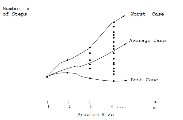
Best, worst, and average-case complexity
Linear search
def linear_search(my_item, items):
    for position, item in enumerate(items):
        if my_item == item:
            return position
Worst case: T(n) = n
Average case: T(n) = 1/2 ⋅ n
Best case: T(n) = 1
T(n) = O(n)
How can we compare two functions?
We can use Asymptotic notation
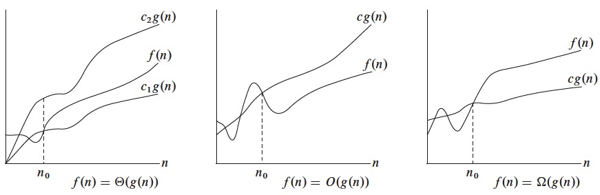
Asymptotic notation
The Big Oh Notation
Asymptotic upper bound
O(g(n)) = {f(n): there exist positive constants c and n0 such that 0 ≤ f(n) ≤ c⋅g(n) for all n ≥ n0}
T(n) ∈ O(g(n))
or
T(n) = O(g(n))
Ω-Notation
Asymptotic lower bound
Ω(g(n)) = {f(n): there exist positive constants c and n0 such that 0 ≤ c⋅g(n) ≤ f(n) for all n ≥ n0}
T(n) ∈ Ω(g(n))
or
T(n) = Ω(g(n))
Θ-Notation
Asymptotic tight bound
Θ(g(n)) = {f(n): there exist positive constants c1, c2 and n0 such that 0 ≤ c1⋅g(n) ≤ f(n) ≤ c2⋅g(n) for all n ≥ n0}
T(n) ∈ Θ(g(n))
or
T(n) = Θ(g(n))
Graphic examples of the Θ, O and Ω notations
Examples
3⋅n2 - 100⋅n + 6 = O(n2),
because we can choose c = 3 and
3⋅n2 > 3⋅n2 - 100⋅n + 6
100⋅n2 - 70⋅n - 1 = O(n2),
because we can choose c = 100 and
100⋅n2 > 100⋅n2 - 70⋅n - 1
3⋅n2 - 100⋅n + 6 ≈ 100⋅n2 - 70⋅n - 1
Linear search
Linear search (Villarriba version):
T(n) = O(n)
Linear search (Villabajo version)
def linear_search(my_item, items):
    for position, item in enumerate(items):
        print('position – {0}, item – {0}'.format(position, item))
        print('Compare two items.')
        if my_item == item:
            print('Yeah!!!')
            print('The end!')
            return position
T(n) = O(3⋅n + 2) = O(n)
Speed of "Villarriba version" ≈ Speed of "Villabajo version"
Types of Order
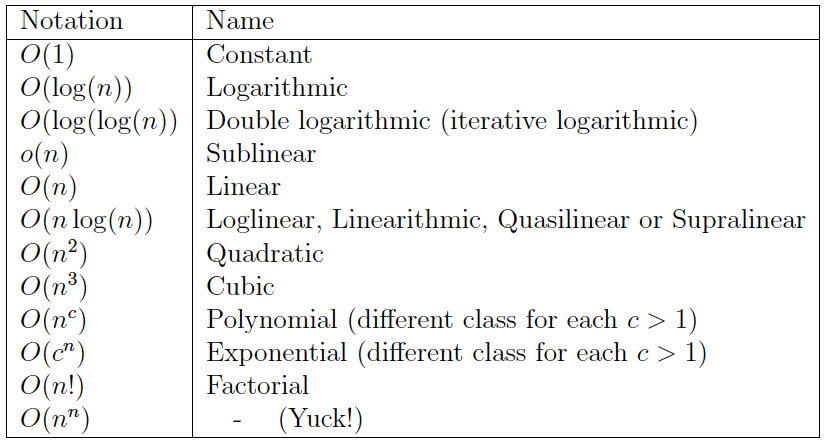
However, all you really need to understand is that:
n! ≫ 2n ≫ n3 ≫ n2 ≫ n⋅log(n) ≫ n ≫ log(n) ≫ 1
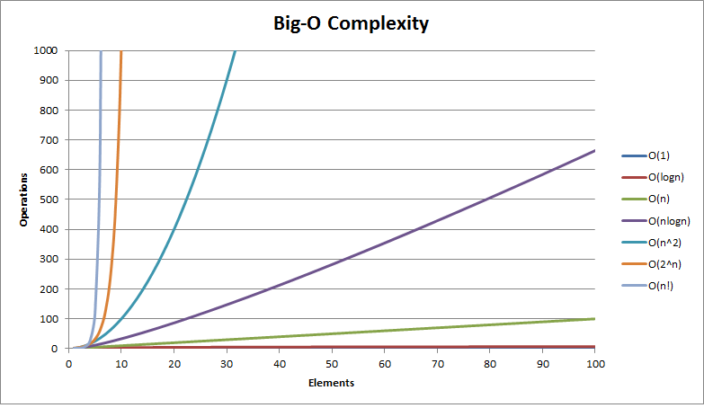
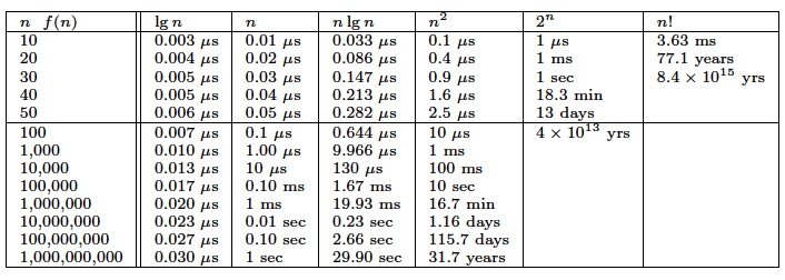
The Big Oh complexity for different functions
Growth rates of common functions measured in nanoseconds
Each operation takes one nanosecond (10-9 seconds).
CPU ≈ 1 GHz
Binary search
def binary_search(seq, t):
    min = 0; max = len(seq) - 1
    while 1:
        if max < min:
            return -1
        m = (min + max) / 2
        if seq[m] < t:
            min = m + 1
        elif seq[m] > t:
            max = m - 1
        else:
            return m
T(n) = O(log(n))
Practical usage
Add DB “index”
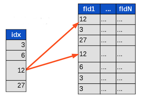
Search with index vs Search without index
Binary search vs Linear search
O(log(n)) vs O(n)
How can you quickly find out complexity?
O(?)

On the basis of the issues discussed here, I propose that members of SIGACT, and editors of computer science and mathematics journals, adopt the O, Ω and Θ notations as defined above, unless a better alternative can be found reasonably soon.
D. E. Knuth, "Big Omicron and Big Omega and BIg Theta", SIGACT News, 1976.
Benchmarks
or
Asymptotic analysis?
Use both approaches!
Summary
- We want to predict running time of an algorithm.
- Summarize all possible inputs with a single “size” parameter n.
- Many problems with “empirical” approach (measure lots of test cases with various n and then extrapolate).
- Prefer “analytical” approach.
- To select best algorithm, compare their T(n) functions.
- To simplify this comparision “round” the function using asymptotic (“big-O”) notation
- Amazing fact: Even though asymptotic complexity analysis makes many simplifying assumptions, it is remarkably useful in practice: if A is O(n3) and B is O(n2) then B really will be faster than A, no matter how they’re implemented.
Links
Books:
- “Introduction To Algorithms, Third Edition”, 2009, by Thomas H. Cormen, Charles E. Leiserson, Ronald L. Rivest and Clifford Stein
- “The Algorithm Design Manual, Second Edition”, 2008, by Steven S. Skiena
Other:
- “Algorithms: Design and Analysis” by Tim Roughgarden
https://www.coursera.org/course/algo - Big-O Algorithm Complexity Cheat Sheet
http://bigocheatsheet.com/
The end
Thank you for attention!
- Vasyl Nakvasiuk
- Email: vaxxxa@gmail.com
- Twitter: @vaxXxa
- Github: vaxXxa
This presentation:
Source: https://github.com/vaxXxa/talks